ShardTensor

Domain parallelism for high-resolution science

Corey Adams, Peter Harrington, Akshay Subramaniam, Mohammad Shoaib Abbas, Jaideep Pathak, Negin Sobhani, Dallas Foster, Mike Pritchard, Sanjay Choudhry
NVIDIA · AI4S Workshop @ SC26, Chicago

AI for Science is working

Proteins Structure prediction competitive with experiment AlphaFold · Nature 2021

Weather Global medium-range forecasts that beat operational numerical systems GraphCast · Science 2023; Pangu-Weather · Nature 2023

Fusion Magnetic control of tokamak plasmas by deep reinforcement learning Nature 2022

Materials Deep learning at scale for materials discovery, and autonomous synthesis labs Nature 2023 (×2)

Fluids Machine-learning-accelerated computational fluid dynamics PNAS 2021

Medicine Dermatologist-level classification of skin cancer Nature 2017

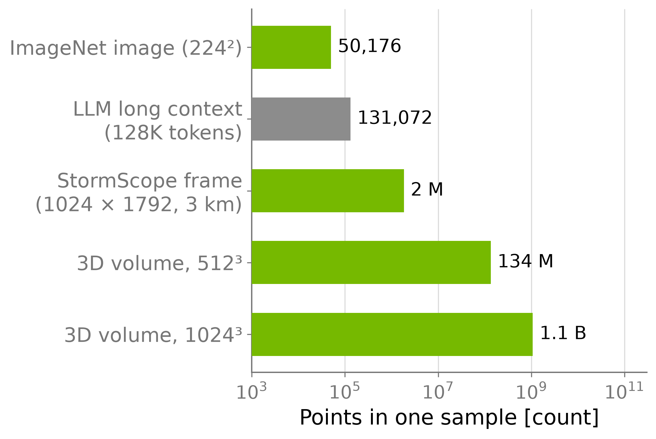
Science wants resolution

Resolution is where discoveries are made:

• the first image of a black hole
• atomic-resolution protein structures from cryo-EM
• a petavoxel map of human cortex
• meter-scale clouds that drive climate sensitivity

one scientific sample is often far larger than one language-model sample.

But, training an AI for Science model at true resolution is hard

torch.cuda.OutOfMemoryError: CUDA out of memory.

Current parallelism was built for different problems

The parallelism toolbox came from image and language models

Method	What it splits	Built for
Data parallel (Horovod, DDP)	the batch: one or more samples per GPU	more data per step
Fully sharded (FSDP, ZeRO)	weights, gradients, optimizer state	models too big for one GPU
Tensor parallel	each weight matrix	layers too big for one GPU
Pipeline parallel	groups of layers	very deep models
Context / sequence parallel	tokens, inside attention	long text; transformers only

Every tool assumes either that one sample fits on a GPU, or that the model is a transformer.

Why does resolution become memory?

\( z = W x + b \)

→

→

\(W\)

\(W:\; N \times N\)

\(x:\; P \times N\)

\(z:\; P \times N\)

one H100: 80 GB

weights: 1 MB

Variable

Source

Floats (fp32 = 4 B)

When

\( x, z \)

Active data

\( P \times N \)

Train & infer

\( W, b \)

Model weights

\( N^2 \)

Train & infer

\( \nabla W, m, v \)

Training buffers

\( 3 \times N^2 \)

Train only

\( \text{saved } x \)

Saved activations

\( P \times N \)

Train only

Why does resolution become memory?

\( z = W x + b \)

→

→

\(W\)

\(W:\; N \times N\)

\(x:\; P \times N\)

\(z:\; P \times N\)

one H100: 80 GB

weights: 1 MB

Variable

Source

Floats (fp32 = 4 B)

When

\( x, z \)

Active data

\( P \times N \)

Train & infer

\( W, b \)

Model weights

\( N^2 \)

Train & infer

\( \nabla W, m, v \)

Training buffers

\( 3 \times N^2 \)

Train only

\( \text{saved } x \)

Saved activations

\( P \times N \)

Train only

Why does resolution become memory?

\( z = W x + b \)

→

→

\(W\)

\(W:\; N \times N\) (+ buffers)

\(\nabla W\)
\(m, v\)

\(x:\; P \times N\)

\(z:\; P \times N\)

one H100: 80 GB

weights + buffers: 4 MB

Variable

Source

Floats (fp32 = 4 B)

When

\( x, z \)

Active data

\( P \times N \)

Train & infer

\( W, b \)

Model weights

\( N^2 \)

Train & infer

\( \nabla W, m, v \)

Training buffers

\( 3 \times N^2 \)

Train only

\( \text{saved } x \)

Saved activations

\( P \times N \)

Train only

Why does resolution become memory?

\( z = W x + b \qquad\Rightarrow\qquad \tfrac{\partial L}{\partial W} = (\tfrac{\partial L}{\partial z})^{\!\top} x \)

→

→

\(W\)

\(W:\; N \times N\) (+ buffers)

\(\nabla W\)
\(m, v\)

\(x:\; P \times N\)

\(z:\; P \times N\)

saved for backward

one H100: 80 GB

weights + buffers: 4 MB

Variable

Source

Floats (fp32 = 4 B)

When

\( x, z \)

Active data

\( P \times N \)

Train & infer

\( W, b \)

Model weights

\( N^2 \)

Train & infer

\( \nabla W, m, v \)

Training buffers

\( 3 \times N^2 \)

Train only

\( \text{saved } x \)

Saved activations

\( P \times N \)

Train only

Why does resolution become memory?

\( z = W x + b \qquad\Rightarrow\qquad \tfrac{\partial L}{\partial W} = (\tfrac{\partial L}{\partial z})^{\!\top} x \)

→

→

\(W\)

\(W:\; N \times N\) (+ buffers)

\(\nabla W\)
\(m, v\)

\(x:\; 64^3 \times 512\)

\(z:\; 64^3 \times 512\)

saved for backward

one H100: 80 GB

537 MB

weights + buffers: 4 MB

Variable

Source

Floats (fp32 = 4 B)

Total

When

\( x, z \)

Active data

\( 64^3 \times 512 \)

537 MB

Train & infer

\( W, b \)

Model weights

\( 512^2 \)

1 MB

Train & infer

\( \nabla W, m, v \)

Training buffers

\( 3 \times 512^2 \)

3 MB

Train only

\( \text{saved } x \)

Saved activations

\( 64^3 \times 512 \)

537 MB

Train only

Why does resolution become memory?

\( z = W x + b \qquad\Rightarrow\qquad \tfrac{\partial L}{\partial W} = (\tfrac{\partial L}{\partial z})^{\!\top} x \)

→

→

\(W\)

\(W:\; N \times N\) (+ buffers)

\(\nabla W\)
\(m, v\)

\(x:\; 128^3 \times 512\)

\(z:\; 128^3 \times 512\)

saved for backward

one H100: 80 GB

4 GB

weights + buffers: 4 MB

Variable

Source

Floats (fp32 = 4 B)

Total

When

\( x, z \)

Active data

\( 128^3 \times 512 \)

4 GB

Train & infer

\( W, b \)

Model weights

\( 512^2 \)

1 MB

Train & infer

\( \nabla W, m, v \)

Training buffers

\( 3 \times 512^2 \)

3 MB

Train only

\( \text{saved } x \)

Saved activations

\( 128^3 \times 512 \)

4 GB

Train only

Why does resolution become memory?

\( \text{fp32 (4 B/val):} \quad 4\,\text{B} \times L \times (\; \underbrace{4N^2}_{W \text{ + buffers}} \;+\; \underbrace{P N}_{\text{saved } x} \;) \)

\(W_{1}\)

\(W_{2}\)

\(W_{3}\)

\(W_{4}\)

\(W_{5}\)

\(W_{6}\)

\(W_{7}\)

\(W_{8}\)

\(W_{9}\)

\(W_{10}\)

\(W_{11}\)

\(W_{12}\)

\(W_{13}\)

\(W_{14}\)

\(W_{15}\)

\(W_{16}\)

\(W_{17}\)

\(W_{18}\)

\(W_{19}\)

\(W_{20}\)

one H100: 80 GB

86 GB

weights + buffers: 84 MB

Variable

Source

Floats (fp32 = 4 B)

Total

When

\( x, z \)

Active data

\( 128^3 \times 512 \)

4 GB

Train & infer

\( W, b \)

Model weights

\( 20 \times 512^2 \)

21 MB

Train & infer

\( \nabla W, m, v \)

Training buffers

\( 3 \times 20 \times 512^2 \)

63 MB

Train only

\( x_1 \dots x_L \)

Saved activations

\( 20 \times 128^3 \times 512 \)

86 GB

Train only

On one GPU, every fix has a cost

as is

86 GB

fp32, 20 layers

half precision

43 GB

only 2×, once;
less dynamic range

half the layers

43 GB

a smaller,
less accurate model

checkpoint:
save 1 layer in 4

21 GB

recompute the rest
in backward: slower

downsample
to 64³

11 GB

loses the
fine detail

Every single-GPU fix trades away speed, model size, or resolution.

Four GPUs: what can we split?

Shard the weights (FSDP, tensor parallel)

one sample: 128³ points

GPU 0

86 GB

GPU 1

¼ of W: 5 MB

GPU 2

¼ of W: 5 MB

GPU 3

¼ of W: 5 MB

The weights were only 21 MB. The saved inputs still sit on one GPU.

Four GPUs: what can we split?

Split the batch (data parallel, DDP)

one sample: 128³ points

GPU 0

86 GB

GPU 1

idle

GPU 2

idle

GPU 3

idle

Each GPU needs a whole sample. At batch size 1, there is nothing left to split.

Four GPUs: what can we split?

Split the sample (domain parallel)

one sample: 128³ points

GPU 0

21 GB

GPU 1

21 GB

GPU 2

21 GB

GPU 3

21 GB

Each GPU holds a quarter of the points, and a full copy of the small weights.

Domain parallelism today: proven, but bespoke

Where	What it splits	The catch
Classical HPC: CFD, climate, molecular dynamics	the simulation domain, for decades	solvers, not ML models
Ring Attention, DeepSpeed Ulysses	the token sequence	attention and transformers only
Makani (weather), Transolver++ (CFD)	the spatial domain	written into one model
DistDL	layers, over MPI	rebuild the model; fixed partitions
PyTorch DTensor	any tensor	built for weights: even, static shapes
JAX shard_map	anything	you compose every operation by hand

Missing: a general tool where your model runs unchanged.

ShardTensor

What is ShardTensor?

One logical tensor, uneven pieces across GPUs

GPU 0

local shard

34k pts

GPU 1

local shard

28k pts

GPU 2

local shard

36k pts

GPU 3

local shard

24k pts

Why it matters:

• Your model stays a 1-GPU model — no parallel code in forward()

• Each GPU's piece can have a different size (convolutions, meshes, point clouds)

• Exact single-GPU math — halos, all-reduces, and rings run automatically

• Composes with DDP & FSDP2 for data × domain (× model)

Extends PyTorch's DTensor for scientific data

PyTorch DTensor

ShardTensor

Built for

Model weights

High-res inputs & activations

Chunk sizes

Even only (torch.chunk)

Uneven per GPU (tracks per-rank shapes)

Shapes

Static across steps

Dynamic through layers

Operations

Generic tensor redistributions

Halo, ring, all-reduce + DTensor fallback

Model code

distribute_module

Unchanged nn.Module

What DDP did for data parallelism, ShardTensor does for domain parallelism — open source in physicsnemo.domain_parallel.

In practice: two lines change

from torch.distributed.device_mesh import init_device_mesh
from torch.nn.parallel import DistributedDataParallel as DDP
from torch.distributed.tensor import Shard
from physicsnemo.domain_parallel import scatter_tensor, sync_module_over_mesh

mesh = init_device_mesh("cuda", (16, 2), mesh_dim_names=("data", "domain"))
model = MyModel().cuda()  # your model, unchanged
model = DDP(model, process_group=mesh["data"].get_group())
loss_fn(model(x), y).backward()

MyModel is not rewritten. The ShardTensor input triggers domain-parallel dispatch inside every layer, forward and backward.

In practice: two lines change

from torch.distributed.device_mesh import init_device_mesh
from torch.nn.parallel import DistributedDataParallel as DDP
from torch.distributed.tensor import Shard
from physicsnemo.domain_parallel import scatter_tensor, sync_module_over_mesh

mesh = init_device_mesh("cuda", (16, 2), mesh_dim_names=("data", "domain"))
model = MyModel().cuda()  # your model, unchanged
# 1. Make the weights agree across GPUs that share a sample
sync_module_over_mesh(model, mesh["domain"])
model = DDP(model, process_group=mesh["data"].get_group())
# 2. Split each input sample along its height axis
x = scatter_tensor(x, src, mesh["domain"], (Shard(2),))
loss_fn(model(x), y).backward()

MyModel is not rewritten. The ShardTensor input triggers domain-parallel dispatch inside every layer, forward and backward.

Under the hood: dispatch, layer by layer

Your model, written for one GPU

Conv

Norm

→

MLP

→

Attention

→

MLP

→

Loss

→

Under the hood: dispatch, layer by layer

Each operation is dispatched as it runs

Conv

Norm

→

MLP

→

Attention

→

MLP

→

Loss

→

halo

all-reduce

local

ring

local

all-reduce

Under the hood: dispatch, layer by layer

…and routed across the GPUs that share the sample

Conv

Norm

→

MLP

→

Attention

→

MLP

→

Loss

→

halo

all-reduce

local

ring

local

all-reduce

GPU 0

GPU 1

GPU 2

GPU 3

↕

↕

↕

↕

↕

↕

Linear layers, MLPs, and activations

GPU 0

GPU 1

GPU 2

GPU 3

W

W

W

W

z = Wx + b ✓

z = Wx + b ✓

z = Wx + b ✓

z = Wx + b ✓

Each point is updated from its own features alone.

Each GPU runs the layer on its own piece.

No communication between GPUs. Only layers that mix points need to talk.

Convolutions and local stencils

A convolution updates each cell from its local neighborhood (e.g. 3 × 3).

Convolutions and local stencils

GPU 0

GPU 1

?

?

?

At a GPU boundary, part of the neighborhood sits on the adjacent GPU.

Convolutions and local stencils

GPU 0

GPU 1

Halo exchange: each GPU copies a thin boundary strip from its neighbor.

Normalization, pooling, and losses

 GPU 0

 GPU 1

 GPU 2

 GPU 3

Σx, Σx² on 0

Σx, Σx² on 1

Σx, Σx² on 2

Σx, Σx² on 3

Normalization and loss layers need statistics over the whole sample. Each GPU sums its local shard.

Normalization, pooling, and losses

 GPU 0

 GPU 1

 GPU 2

 GPU 3

Σx, Σx² on 0

Σx, Σx² on 1

Σx, Σx² on 2

Σx, Σx² on 3

mean, var

mean, var

mean, var

mean, var

mean, var

All-reduce: combine the partial sums across GPUs…

Normalization, pooling, and losses

 GPU 0

 GPU 1

 GPU 2

 GPU 3

mean, var

mean, var

mean, var

mean, var

mean, var

…so every GPU gets the exact global statistics. Only a few scalars move.

Self-attention and global layers

 GPU 0

Q₀

 GPU 1

Q₁

 GPU 2

Q₂

 GPU 3

Q₃

K₀ V₀

K₁ V₁

K₂ V₂

K₃ V₃

Q₀

K₀

Q₁

K₁

Q₂

K₂

Q₃

K₃

 one GPU

Self-attention mixes every point with every other point (all pairs of Q and K, V).

H. Liu, M. Zaharia, P. Abbeel, “Ring Attention with Blockwise Transformers for Near-Infinite Context,” arXiv:2310.01889 (2023)

Self-attention and global layers

 GPU 0

Q₀

 GPU 1

Q₁

 GPU 2

Q₂

 GPU 3

Q₃

K₀ V₀

K₁ V₁

K₂ V₂

K₃ V₃

Q₀

K₀

Q₁

K₁

Q₂

K₂

Q₃

K₃

 one GPU

Ring attention: each GPU keeps its own queries Q_i and starts with its local K_i, V_i.

H. Liu, M. Zaharia, P. Abbeel, “Ring Attention with Blockwise Transformers for Near-Infinite Context,” arXiv:2310.01889 (2023)

Self-attention and global layers

 GPU 0

Q₀

 GPU 1

Q₁

 GPU 2

Q₂

 GPU 3

Q₃

K₀ V₀

K₁ V₁

K₂ V₂

K₃ V₃

Q₀

K₀

Q₁

K₁

Q₂

K₂

Q₃

K₃

 one GPU

Ring attention (step 1/4): compute attention block while passing K, V to the next GPU.

H. Liu, M. Zaharia, P. Abbeel, “Ring Attention with Blockwise Transformers for Near-Infinite Context,” arXiv:2310.01889 (2023)

Self-attention and global layers

 GPU 0

Q₀

 GPU 1

Q₁

 GPU 2

Q₂

 GPU 3

Q₃

K₀ V₀

K₁ V₁

K₂ V₂

K₃ V₃

Q₀

K₀

Q₁

K₁

Q₂

K₂

Q₃

K₃

 one GPU

Ring attention (step 2/4): compute attention block while passing K, V to the next GPU.

H. Liu, M. Zaharia, P. Abbeel, “Ring Attention with Blockwise Transformers for Near-Infinite Context,” arXiv:2310.01889 (2023)

Self-attention and global layers

 GPU 0

Q₀

 GPU 1

Q₁

 GPU 2

Q₂

 GPU 3

Q₃

K₀ V₀

K₁ V₁

K₂ V₂

K₃ V₃

Q₀

K₀

Q₁

K₁

Q₂

K₂

Q₃

K₃

 one GPU

Ring attention (step 3/4): compute attention block while passing K, V to the next GPU.

H. Liu, M. Zaharia, P. Abbeel, “Ring Attention with Blockwise Transformers for Near-Infinite Context,” arXiv:2310.01889 (2023)

Self-attention and global layers

 GPU 0

Q₀

 GPU 1

Q₁

 GPU 2

Q₂

 GPU 3

Q₃

K₀ V₀

K₁ V₁

K₂ V₂

K₃ V₃

Q₀

K₀

Q₁

K₁

Q₂

K₂

Q₃

K₃

 one GPU

Ring attention (step 4/4): compute attention block while passing K, V to the next GPU.

H. Liu, M. Zaharia, P. Abbeel, “Ring Attention with Blockwise Transformers for Near-Infinite Context,” arXiv:2310.01889 (2023)

Self-attention and global layers

 GPU 0

Q₀

 GPU 1

Q₁

 GPU 2

Q₂

 GPU 3

Q₃

K₀ V₀

K₁ V₁

K₂ V₂

K₃ V₃

Q₀

K₀

Q₁

K₁

Q₂

K₂

Q₃

K₃

 

Ring attention: after 4 steps, every GPU has attended to the full sample.

H. Liu, M. Zaharia, P. Abbeel, “Ring Attention with Blockwise Transformers for Near-Infinite Context,” arXiv:2310.01889 (2023)

Three patterns cover most scientific models

Layers	Communication	What moves
Linear, MLP, activations	none	nothing
Convolution, neighborhood attention, graph message passing	halo exchange	a thin edge from each neighbor
Normalization, pooling, loss	all-reduce	a few statistics per GPU
Full attention	ring	keys and values, overlapped with compute

Each gives the same answer as one GPU.

Extending ShardTensor: your own operation

import torch, torch.distributed as dist
from torch.distributed.tensor import Replicate
from physicsnemo.domain_parallel import ShardTensor

def sharded_dot(func, types, args, kwargs):
    x, y = args
    out = torch.dot(x.to_local(), y.to_local())  # each GPU: its own piece
    dist.all_reduce(out, group=x._spec.mesh.get_group())  # sum over GPUs
    return ShardTensor.from_local(out, x._spec.mesh, (Replicate(),))
ShardTensor.register_function_handler(torch.dot, sharded_dot)

Register handlers for Python functions, torch.library.custom_op kernels, or low-level aten ops — intercept and parallelize user code at whatever level fits your model.

Two axes of parallelism: data × domain

Data parallel: one sample per GPU

data axis (DDP or FSDP2): one sample per group →

… ×16

 GPU 0

 GPU 1

 GPU 2

 GPU 3

DDP and FSDP2 scale across samples. Each GPU must still hold a whole sample.

Two axes of parallelism: data × domain

Data × domain: init_device_mesh("cuda", (16, 2))

data axis (DDP or FSDP2): one sample per group →

… ×16

domain axis
(ShardTensor):
one sample,
2 GPUs ↓

 GPU 0

 GPU 1

↕

 GPU 2

 GPU 3

↕

 GPU 4

 GPU 5

↕

 GPU 6

 GPU 7

↕

ShardTensor splits each group's sample across a second axis. With FSDP2 the weights are sharded too: data × domain × model.

Does it scale?

A vision transformer on a billion-voxel volume

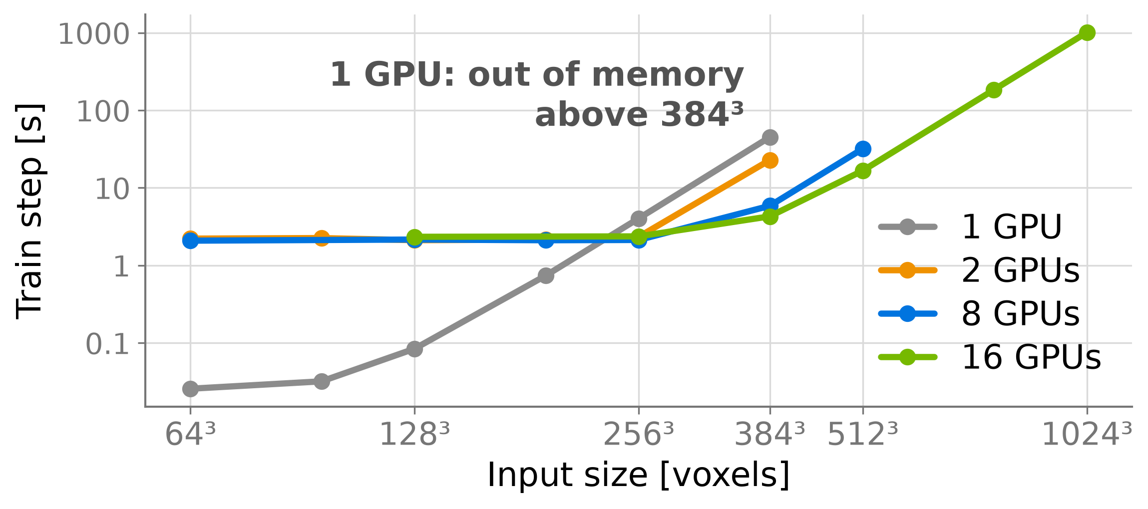
One GPU stops at 384³. 16 GPUs train 1024³ = 1.07 billion points, and run 384³ 10.5× faster.

Large problems scale nearly linearly

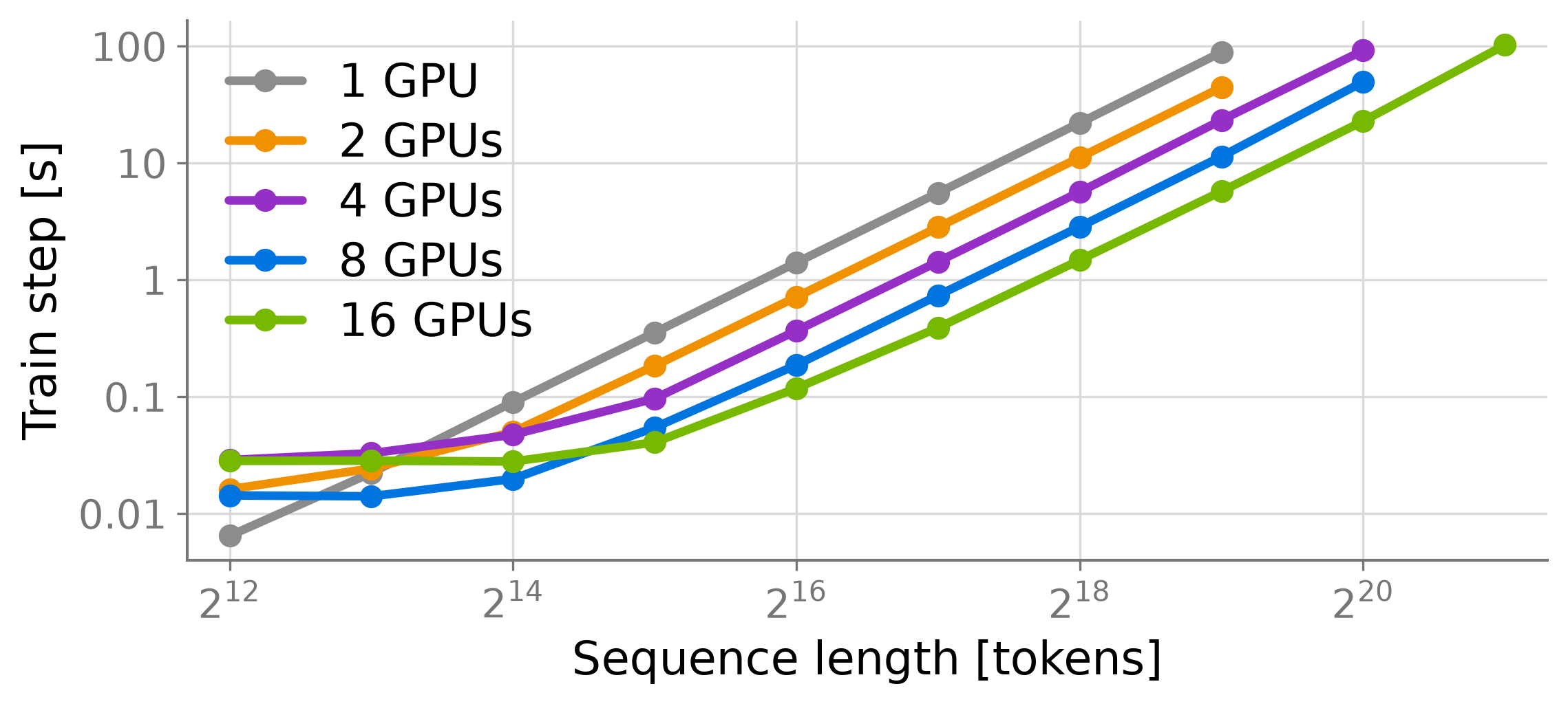
Ring attention training latency. At 2¹⁹ tokens, 16 GPUs are 97% efficient (96% for inference).

Inference at high resolution is faster too

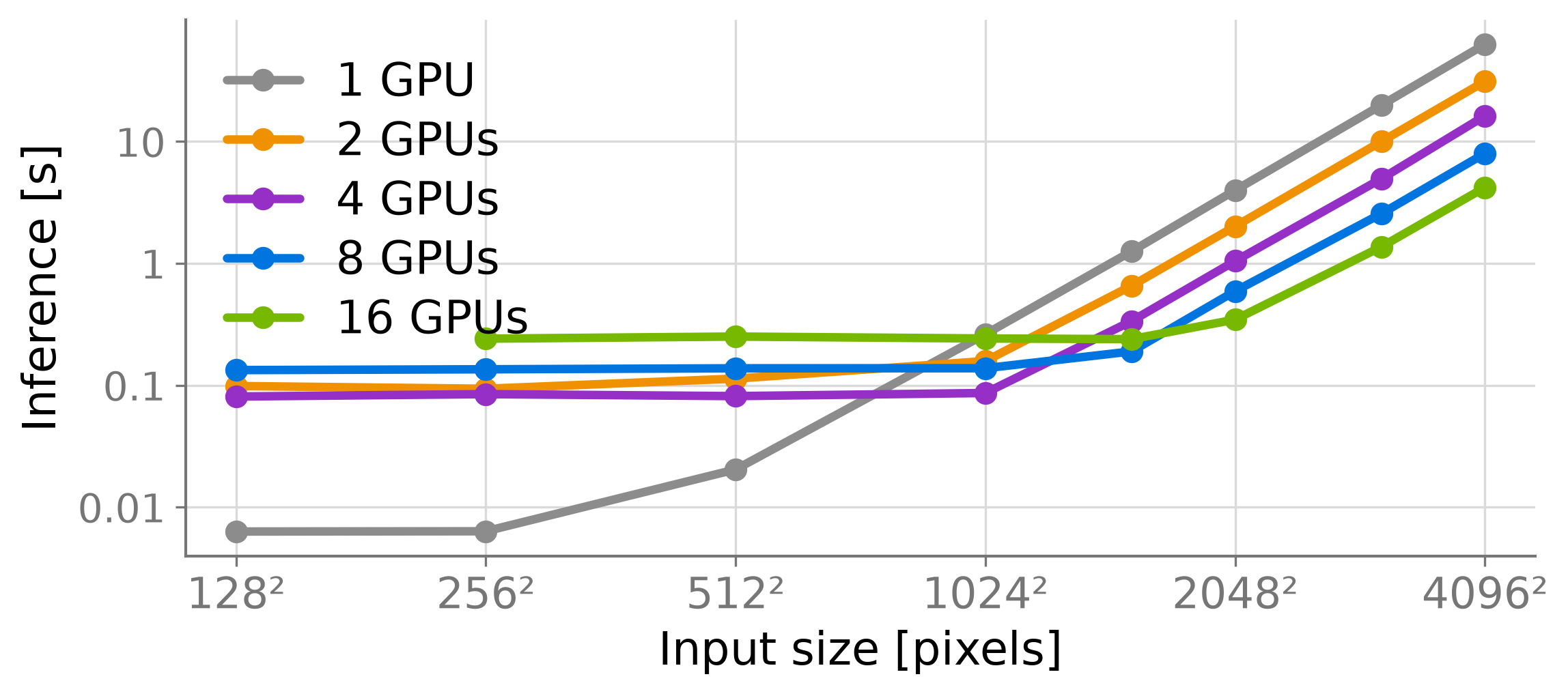
ViT inference on 2D data: 16 GPUs are 14.9× faster than one at 4096².

Dispatch overhead is small; torch.compile cuts it

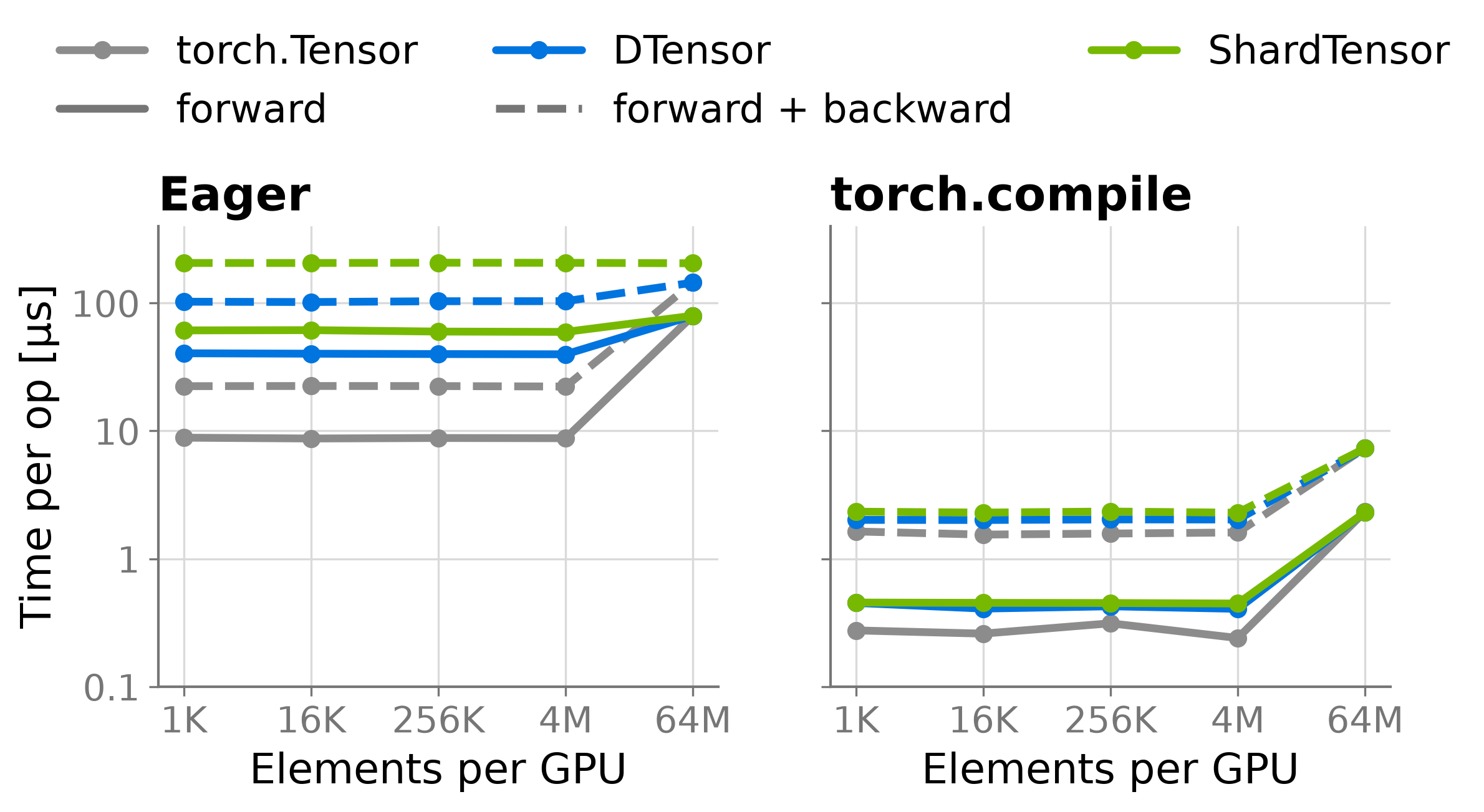
At scientific resolutions, ~60 µs of eager dispatch is small next to GPU kernel time. torch.compile cuts it 134×, to 0.45 µs.

What it enables

StormScope: storms at 3 km across the US

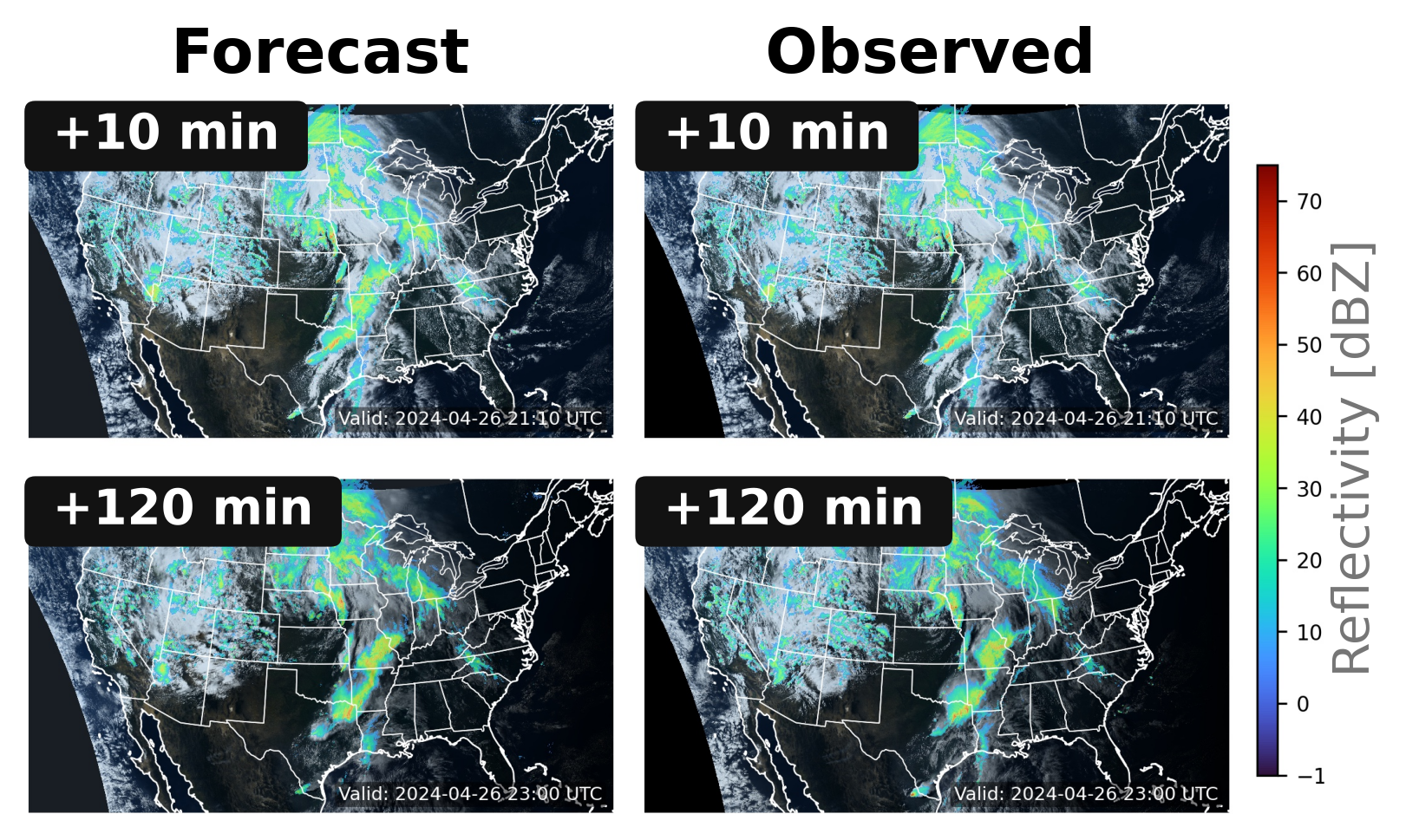
• Storms are kilometer-scale cells driven by weather systems thousands of km across. A forecast needs both.
• 1024 × 1792 grid at 3 km; satellite + radar; 2-hour diffusion forecast; 195 M parameters.
• Peak memory ≈ 114 GB > 80 GB on one H100.
• Trained on 32 H100s: 16 data-parallel groups × 2 GPUs per sample.

Left: forecast. Right: what happened. Without domain parallelism: a coarser grid or a smaller region.

Atomistic simulation: more atoms, same potential

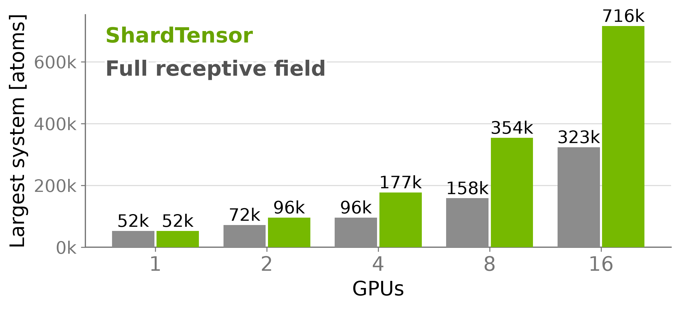
MACE on quartz (SiO₂) via NVIDIA ALCHEMI: 52 k atoms on 1 GPU → 716 k on 16 (vs. 323 k when copying the full multi-hop receptive field).

Aerodynamics: same accuracy at 8× the points

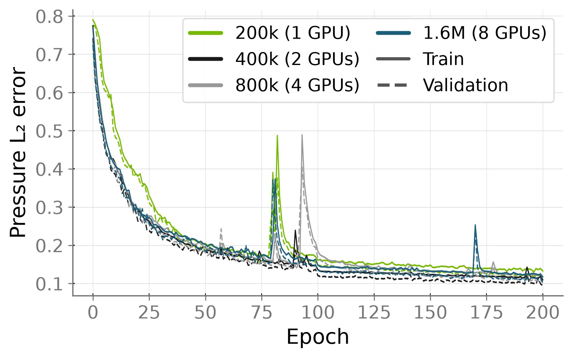
• Transolver on DrivAerML car aerodynamics, volume fields.
• 200 k points per GPU; 1, 2, 4, 8 GPUs per sample → up to 1.6 M points.
• All resolutions converge to the same pressure error (L₂ ≈ 0.10–0.12).
• Data loading and preprocessing are domain parallel too.

Domain-parallel training is as stable as single-GPU training, and combines with data parallelism.

Should you use ShardTensor?

• One sample does not fit, or one sample is too slow. If the batch can still be split, data parallelism is faster.
• Big operations. Eager dispatch costs ~60 µs per op; torch.compile cuts it to ~0.45 µs.
• Pieces that stay large. When each GPU’s piece is small next to the halo it exchanges, scaling drops.
• Fast interconnect. Results here are on NVLink (GB200 NVL72, H100 nodes).
• Operator coverage. Unregistered PyTorch ops fall back to DTensor or a handler you write. Tested to 16 GPUs per sample.

How to use ShardTensor

1. Install NVIDIA PhysicsNeMo

pip install "nvidia-physicsnemo[cu13]"

from physicsnemo.domain_parallel import (
    ShardTensor,
    scatter_tensor,
    sync_module_over_mesh,
)

Coming soon: PhysicsNeMo is splitting key functionality into standalone libraries — pip install physicsnemo-domain-parallel will soon be available.

2. Install the coding-agent skill

Clone the repo and link skills/physicsnemo-shard-tensor into your agent’s skills directory (Claude Code, Codex, Cursor, OpenCode):

git clone --depth 1 https://github.com/NVIDIA/physicsnemo
mkdir -p ~/.claude/skills ~/.codex/skills
ln -s "$PWD/physicsnemo/skills/physicsnemo-shard-tensor" \
      ~/.claude/skills/physicsnemo-shard-tensor

• Wires DeviceMesh + scatter_tensor into your script without touching your nn.Module
• Configures DDP or FSDP2 + domain parallelism, custom op handlers, and torchrun gradient tests

Conclusions

Resolution should be a scientific choice, not a GPU-memory limit.

• For scientific data, memory is dominated by saved inputs, which grow with the points in one sample. Sharding weights or batches does not touch them.
• Domain parallelism splits exactly that dimension. Point-wise layers need no communication; the rest need halos, all-reduces, or rings.
• ShardTensor makes it a two-line change for unmodified PyTorch models, and it already trains a 3 km storm model, larger atomistic systems, and million-point CFD surrogates.

Docs & tutorials: docs.nvidia.com/physicsnemo/latest · Source & examples: github.com/NVIDIA/physicsnemo (physicsnemo/domain_parallel)

Thank you

Questions?

Slides: coreyadams.net/talks/sc26-shardtensor (PDF) · Code: github.com/NVIDIA/physicsnemo